Convolutional Neural Network has been the most popular way for image-related Machine Learning tasks. This article intends to give you a simple yet clear deep dive into the Convolutional operations. We will be covering the following concepts:

• What is convolution operation?
• Kernel, Filter, Receptive Field
• Channel, Width, Number of Layers
• Padding
• Stride

What is convolution operation?

The easiest way to understand the convolution operation is by running the calculation in a spreadsheet. Consider we have a single-colour image, which means we only have 1 colour channel, and 2 dimensions that represents the width and height. We have already discussed the representation of image in this article. For simplicity, let’s consider a 16×16 pixels image that represents by the numbers below.

In its simplest form, the convolution operation is essentially running a SUMPRODUCT operation between the all the pixel groups and the kernel. It slides over the kernel matrix over the raw image pixels, and produce an outcome. Let’s focus on the operation itself, we will explain why that works later on.

Kernel, Filter, Receptive Field

It might be confusing for sometimes for the terminology of the kernel matrix. There are a few terminologies being used to describe this matrix. Usually, it is called the “Kernel”, or it can also be called the “Filter”. In some papers, it is also called the “Receptive Field”. They are equivalently referring to the same thing.

Consider the left most 4 cells of the raw pixel image. The first convolution operation is to do a SUMPRODUCT between and the kernel , and that comes up to 44. Details as below.

Then, we slide the kernel horizontally to the next part of the raw pixels . Again, we compute the SUMPRODUCT between and the kernel , resulting in 54.

This sliding operation continues until all parts of the image have been scanned.

Convolution on RGB images

One details that I found not easy to understand is the convolution of a colour images with RGB channels. It looks intuitive in all the texts but the details are mostly skipped.

Essentially, to run the convolution operation on a 3-channel image, you are running a SUMPRODUCT operation on each channel, and SUM all the outputs together.

Let’s do it step by step. Because the image has 3 channels, our filter will also have 3 channels, where we can map each channel of the filter to the channel of the image. The first step of the convolution operation will be as follow:

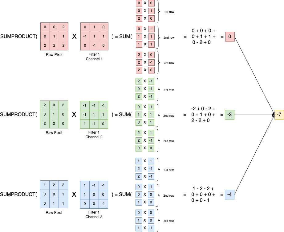
The steps are:

1. Apply the each channel of the filter on the channel of the image respectively. This gives us the by-channel outcome, which is 0, -3, and -4 respectively. (As depicted in the above image)
2. Sum the outcome of each of the channel, then that would be the 1st outcome of the Convolution operation

It is important to note that although the original input has 3 channels, and the filter also has 3 channel, the outcome value is a scalar (1-dimension). This is important because that means the new dimensions after the convolution step is the Outcome width x Outcome height x Number of filters. We will see why this is important in later stage.

This operation will be repeated for each filter. If we have 10 filters, then we will have 10 sets of convolution outcomes. The will be stacked together, which means the outcome of the convolution operation will have 10 channels.

Channels, Width, Number of layers

Now, we have learn the how the Convolution layer works. It’s time to understand some terminologies.

In the above example, we have seen if the input has 3 channels, then the filter will also have 3 channel, and map to a scalar output. However, it might be confusing of the terminology “Number of Channels” in the context of CNN.

A lot of time, when we are describing the architecture that is being used in CNN, we use the “Number of Channels” to describe how many layers of outcome will there be after the convolution operation. It is interchangeable with “Number of layers of filters”, or “The width of convolution layer”.

Let’s take the paper of VGG-16 as an example.

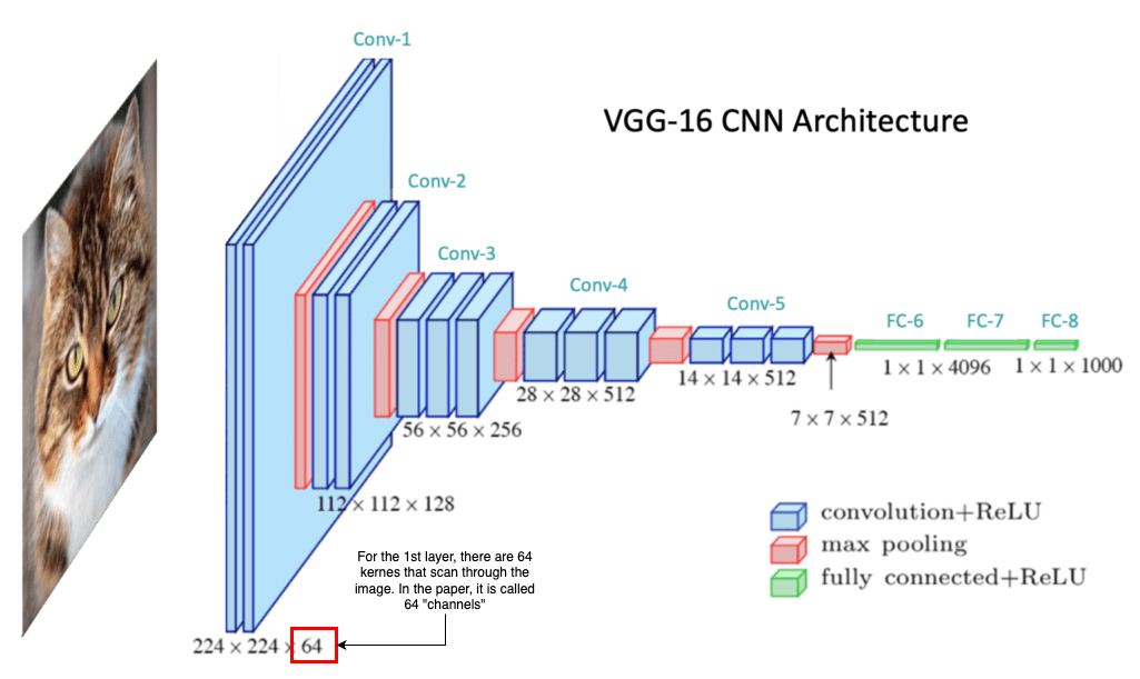
In the VGG-16 paper, the authors used “The width of conv. layers” to describe the number kernels being used in the layer.

… The width of conv. layers (the number of channels) is rather small, starting from 64 in the first layer and then increasing by a factor of 2 after each max-pooling layer, until it reaches 512. … (Source)

Also, in the architecture configuration table, the author describes their ConvNet with naming as “conv(receptive field size)-(number of channels)”. The terminology “Number of channels” also refer the number of kernels being used.

Padding

In the Convolution operation, can observe that the bottom right of the kernel can never be multiplied with the top left of the image pixel.

As illustrated in the above image, we can clearly see that for the kernel , the value of the bottom right corner can never overlap with the top left corner of the image . This will result in information loss during the convolution operation.

To resolve this issue, we can pad the image with a 1 pixel boarder. As illustrated in the above picture, with grey padding, the bottom right of the kernel can be applied to the top left pixel of the image. Hence, this can reduce information loss.

Stride

In the Convolution operation, stride refers to the number of pixels to traverse, both horizontally and vertically, for each “scan”. Up to this point, we have already learnt that the convolution operation works like a scanner. The kernel is used to scan an image in both horizontal and vertical way.

At the beginning, the kernel is positioned to the top left corner and run the SUMPRODUCT. Then, it is moved by 1 pixel, either horizontally or vertically, to scan another groups of pixels. The caveat is that the kernel can choose to move by how many pixels. The parameter to control the movement is called “Stride”.

For example, if we choose stride = 1, the kernel will move and scan every 1 pixel.

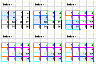
However, if we choose stride = 2, the kernel will move and scan every 2 pixels.

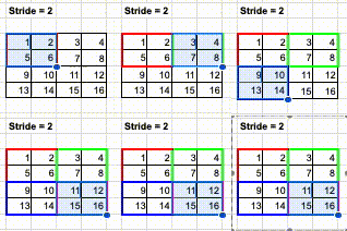
Different stride setting will return a different size of outcome. If the stride is smaller, which means the kernel scans more pixels, then the outcome of convolution will be larger. However, if the stride is larger, which means the kernel scans less pixels, then the outcome of convolution will be smaller.

Understanding PyTorch convolution layer

Now, we should have good understanding on the convolution operation. Of course, we don’t need to implement all the operation details ourselves, as there are plenty of deep learning library that come with Convolution layer out of the box.

Take PyTorch as an example. We can use the torch.nn.Conv2d()function for the convolution operation. Let’s take a look at the function signature:

torch.nn.Conv2d(in_channels, out_channels, kernel_size, stride=1, padding=0, dilation=1, groups=1, bias=True, padding_mode='zeros', device=None, dtype=None)

We can see the Conv2d layer needs to declare the following parameters:

• in_channels: The number of incoming channels. If it is applied on an RGB image, then it would be 3. If it is applied on the subsequent layer after the convolution operations, then this would be the number of kernels of the previous convolution operation.
• out_channels: This is basically the number of kernels to be used. As we have already learnt the number of channels of the outcome is the same as the number of kernels being used in the convolution operation.
• kernel_size: The size of the kernel. It would be a 2×2 kernel, or 3×3, or other combinations. For VGG-16, the author mostly suggest using a 3×3 kernel can improve the results.
• stride: The size of stride for scanning
• padding: The size of padding to be used. We can also define what can be used for padding by specifying padding_mode. By default, 0 is being used for padding.
• For other parameters, please refer to the documentation.

Summary

I hope this article gives a good overview on the convolution operation. I hope it helps you to understand more about the channel dimensions, what is a kernel, and also the use of strides and padding.

Reference

• Very Deep Convolutional Networks For Large-scale Image Recognition (Simonyan and Zisserman, 2015)
• https://learnopencv.com/understanding-convolutional-neural-networks-cnn/