Note: This article is my notes on Statistical Rethinking (2nd Edition) – Chapter 2
Bayesian Model is all about estimating the posterior probability of the parameters. There are 3 categories of techniques to estimate the posterior probability:
- Grid Approximation [This article]
- Quadratic approximation
- Markov Chain Monte Carlo (MCMC)
In this article, we will walk through what is Grid Approximation, its relation to Bayes Theorem, and how to do it in R. This method can also easily translated to Python.
What is Grid Approximation
First, let’s recap the Bayes Theorem in the context of parameter estimation.
![]()
To be more concrete, let’s consider a case where we are flipping a coin. The outcome could be either head (![]() ) or tail (
) or tail (![]() ). We define the probability
). We define the probability ![]() is the probability of getting head (
is the probability of getting head (![]() ).
).
To fit this outcome into the equation, we have
![]()
In Bayesian context, we see the coin flipping exercise is just a process of generating outcome, based on different probability ![]() of having heads. The question is: we do not know what is the parameter
of having heads. The question is: we do not know what is the parameter ![]() . If the coin is fair, then
. If the coin is fair, then ![]() . What if the coin is not fair? could it be 0.4, 0.3, or 0.1?
. What if the coin is not fair? could it be 0.4, 0.3, or 0.1?
Our task is to estimate this parameter ![]() based on the outcome we observed.
based on the outcome we observed.
The steps of Grid Approximation
Grid Approximation is simply listing out all the possible values of ![]() from 0 to 1, and we do the same process as the formula above:
from 0 to 1, and we do the same process as the formula above:
- Prior (
 ): We assume there is the same chance of having any value from 0 to 1, i.e. Uniform distribution.
 - Likelihood (
 ): For each value of
  , we estimate the probability of seeing
  number of heads within
  trails. Let’s say if we flip it for 10 times, and seeing 3 heads, then
  , and
, and  . What is the probability of seeing this result if we say
  ? This becomes a binomial distribution question.
 - Average Probability of Data (
 ): We average out the probability of seeing heads against all the
  s that we have tested. This is used as normalisation factor.
Our goal is to estimate the posterior distribution of the parameter ![]() , which is the probability of tossing Head of a the coin. Assume we have 9 trials of the toss, and obtain 6 Heads.
, which is the probability of tossing Head of a the coin. Assume we have 9 trials of the toss, and obtain 6 Heads.
The steps of Grid approximation is as follow:
- Define the Grid. This means we decide how many points to use in estimating the posteriors, and then we make a list of parameter values on the grid.
- Compute the value of the prior at each parameter value on the grid
- Compute the likelihood at each parameter value
- Compute the unstandardised posterior at each parameter value, by multiplying the prior by the likelihood
1. Define the grid
# Define the grid - From 0 to 1, with 20 steps
# p is the parameter that use to generate likelihood
p_grid <- seq(from = 0, to = 1, length.out = 20)
p_grid
##  [1] 0.00000000 0.05263158 0.10526316 0.15789474 0.21052632 0.26315789
##  [7] 0.31578947 0.36842105 0.42105263 0.47368421 0.52631579 0.57894737
## [13] 0.63157895 0.68421053 0.73684211 0.78947368 0.84210526 0.89473684
## [19] 0.94736842 1.00000000
2. Define prior
Flat Prior from a to b is defined as
![]()
# Let's assume a flat prior
# For all values of p they have the same probability
# Flat prior = 1 / (1 - 0) = 1
prior <- rep(1, 20)

# We can also try different priors
# prior <- ifelse(p_trid < 0.5, 0, 1)
# prior <- exp(-5 * abs(p_grid - 0.5))

prior
##  [1] 1 1 1 1 1 1 1 1 1 1 1 1 1 1 1 1 1 1 1 1
3. Compute the likelihood at each value in the grid
What is the probability of seeing 6H and 3T in 9 trials, if the probability is given as we defined in p_grid?
likelihood <- dbinom(6, size = 9, prob = p_grid)
likelihood
##  [1] 0.000000e+00 1.518149e-06 8.185093e-05 7.772923e-04 3.598575e-03
##  [6] 1.116095e-02 2.668299e-02 5.292110e-02 9.082698e-02 1.383413e-01
## [11] 1.897686e-01 2.361147e-01 2.666113e-01 2.714006e-01 2.450051e-01
## [16] 1.897686e-01 1.179181e-01 5.026670e-02 8.853845e-03 0.000000e+00
4. Compute the product of likelihood and prior
unstd.posterior <- likelihood * prior
unstd.posterior
##  [1] 0.000000e+00 1.518149e-06 8.185093e-05 7.772923e-04 3.598575e-03
##  [6] 1.116095e-02 2.668299e-02 5.292110e-02 9.082698e-02 1.383413e-01
## [11] 1.897686e-01 2.361147e-01 2.666113e-01 2.714006e-01 2.450051e-01
## [16] 1.897686e-01 1.179181e-01 5.026670e-02 8.853845e-03 0.000000e+00
5. Standardise the posterior, so it sums to 1
posterior <- unstd.posterior / sum(unstd.posterior)
posterior
##  [1] 0.000000e+00 7.989837e-07 4.307717e-05 4.090797e-04 1.893887e-03
##  [6] 5.873873e-03 1.404294e-02 2.785174e-02 4.780115e-02 7.280739e-02
## [11] 9.987296e-02 1.242643e-01 1.403143e-01 1.428349e-01 1.289433e-01
## [16] 9.987296e-02 6.205890e-02 2.645477e-02 4.659673e-03 0.000000e+00
Tabulate all the output
library(dplyr)
##
## Attaching package: 'dplyr'
## The following objects are masked from 'package:stats':
##
##     filter, lag
## The following objects are masked from 'package:base':
##
##     intersect, setdiff, setequal, union

df <- data.frame(p_values = p_grid,
                 prior = prior,
                 likelihood = likelihood,
                 unstd_posterior = unstd.posterior,
                 posterior = posterior)

knitr::kable(df, col.names=c("p", "Prior", "Likelihood", "Unnormalised Posterior", "Posterior")) %>%
kableExtra::kable_paper("hover", full_width = F)| p | Prior | Likelihood | Unnormalised Posterior | Posterior |
|---|---|---|---|---|
| 0.0000000 | 1 | 0.0000000 | 0.0000000 | 0.0000000 |
| 0.0526316 | 1 | 0.0000015 | 0.0000015 | 0.0000008 |
| 0.1052632 | 1 | 0.0000819 | 0.0000819 | 0.0000431 |
| 0.1578947 | 1 | 0.0007773 | 0.0007773 | 0.0004091 |
| 0.2105263 | 1 | 0.0035986 | 0.0035986 | 0.0018939 |
| 0.2631579 | 1 | 0.0111609 | 0.0111609 | 0.0058739 |
| 0.3157895 | 1 | 0.0266830 | 0.0266830 | 0.0140429 |
| 0.3684211 | 1 | 0.0529211 | 0.0529211 | 0.0278517 |
| 0.4210526 | 1 | 0.0908270 | 0.0908270 | 0.0478012 |
| 0.4736842 | 1 | 0.1383413 | 0.1383413 | 0.0728074 |
| 0.5263158 | 1 | 0.1897686 | 0.1897686 | 0.0998730 |
| 0.5789474 | 1 | 0.2361147 | 0.2361147 | 0.1242643 |
| 0.6315789 | 1 | 0.2666113 | 0.2666113 | 0.1403143 |
| 0.6842105 | 1 | 0.2714006 | 0.2714006 | 0.1428349 |
| 0.7368421 | 1 | 0.2450051 | 0.2450051 | 0.1289433 |
| 0.7894737 | 1 | 0.1897686 | 0.1897686 | 0.0998730 |
| 0.8421053 | 1 | 0.1179181 | 0.1179181 | 0.0620589 |
| 0.8947368 | 1 | 0.0502667 | 0.0502667 | 0.0264548 |
| 0.9473684 | 1 | 0.0088538 | 0.0088538 | 0.0046597 |
| 1.0000000 | 1 | 0.0000000 | 0.0000000 | 0.0000000 |
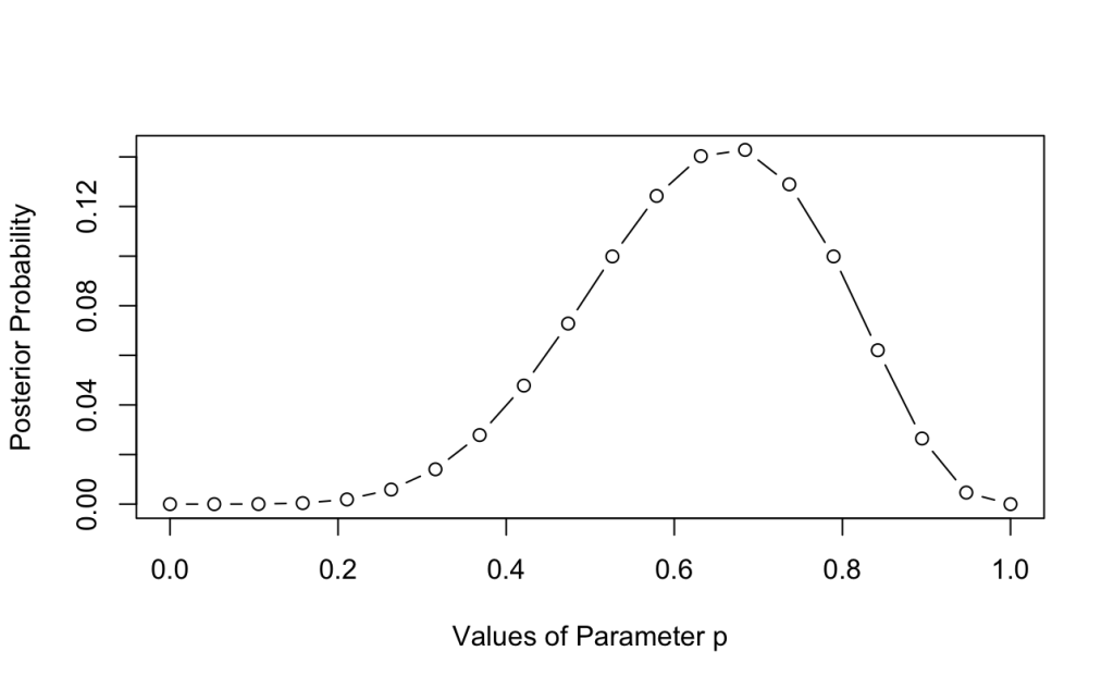
And to visualise the distribution of the posterior probabilities. Based on the posterior distribution, it seems like ![]() is more skewing to the higher side. Maybe from the observation (6 Heads) that we have seen, the coin may not be a fair coin!
is more skewing to the higher side. Maybe from the observation (6 Heads) that we have seen, the coin may not be a fair coin!
plot(p_grid, posterior, type = 'b', lty = 1, xlab = "Values of Parameter p", ylab = "Posterior Probability")
Drawbacks
In simple case, we can use Grid Approximation to estimate the Posterior probability of a parameter. However, if the number of parameters increase, there is a huge challenge of using Grid Approximation. Hence, we will look at Quadratic Approximation and Markov Chain Monte Carlo (MCMC) methods in next examples.

